1. Convolutions

Functionally, a convolution layer usually meant to act as a feature detector. In other words, it is designed to identify signals within a noisy feed. There are roughly three major variations on the theme of improving signal-to-noise ratio: smoothing, change-detection and template-matching. Convolutions play a central role in all three.

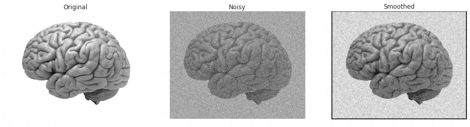
Smoothing is based on the assumption that the true signal effects similarly adjacent samples while the effects of the noise on different samples are pretty much statistically independent. Or alternatively, that the information carried by the signal is concentrated in lower frequencies than the noise. Either way, both perspectives lead to the idea of a filtration by some type of a moving- average. A common approach is to weight each neighbour by its similarity to the point, as measured by a Gaussian radial function:

In change-detection, the target signal is the change in the feed. There are numerous applications for change-detections, such as numerical differentiation and edge-detection. Compared to smoothing, this is a very different problem - but with very similar solutions. This is because the derivative $\lim_{h\rightarrow 0}\frac{f(x+h)-f(x)}{h}$ is a limit of a weighted average, and the discrete approximations of it have the general form of weighted moving averages. This time, the general computation of the weights is a bit tricky, but it's rarely an issue since the applicability of high-order finite differences is limited anyway for the reason that round-off errors quickly shadow truncation errors.

It's very common to apply smoothing as a preliminary step to change-detection, since change detectors are sensitive to noise. In numerical differentiation Savitzky-Golay is such a method, and in edge-detection, the Sobel operator is an example for this type of combination:

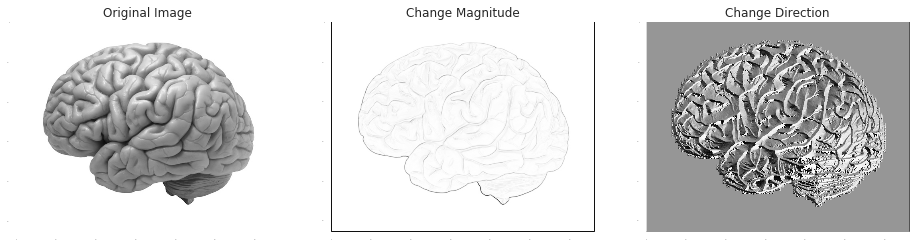
Finally, in template-matching the feed is searched for approximated occurrences of some predetermined template. For example, they can be used to look for appearances of circle-like shapes in an image and alike. Such detectors are often referred to as matched filters.

In general terms, the way they work is by performing a sliding inner-product of the template and the feed. Up to normalization, inner products can be interpreted as a similarity measure between two vectors. So a matched-filter produces localized estimations for local-similarities to its template.

In general terms, the way they work is by performing a sliding inner-product. As an example, let's pick an arbitrary symbol from the Voynich manuscript, and search for the 25 most similar symbols in those 2 pages:

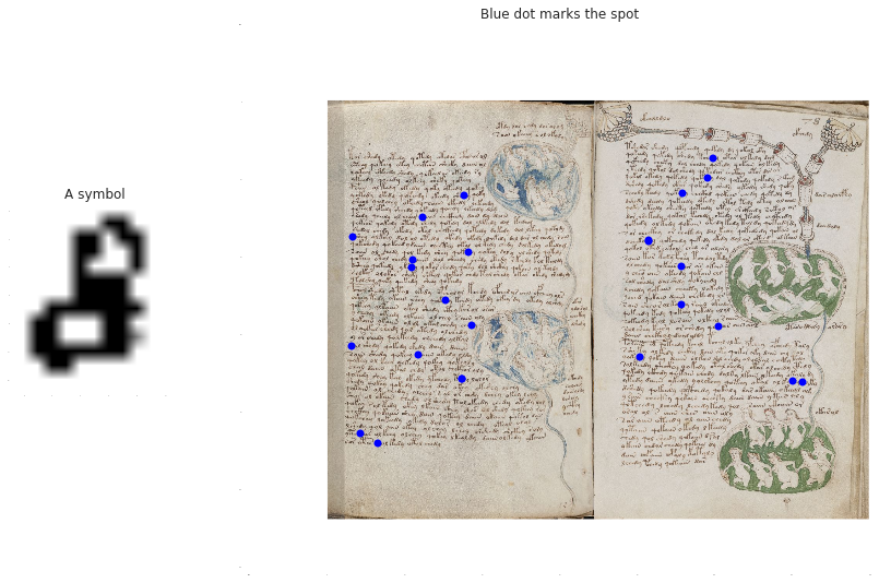
All of the examples so far were linear, and they worked by convolving their feed with some finite impulse response (also known as "kernel", but you can throw a stone and hit 31 completely different things also known as "kernels"). Convolutions will be explained in detail in the next section.

Nonlinear feature-detectors are also a thing, but ConvNets can approximate nonlinear feature-detectors in about the same way feed-forward networks can approximate arbitrary nonlinear functions by chaining adjustable linear functions with fixed nonlinear transformations (ConvNets add subsampling to this mix). Anyway, at least for the meanwhile, nonlinear detectors seem to be much less common in the context of ConvNets.

Functionally, a convolution layer works much like one of those filters above, with one important twist: its impulse response is not "designed" or "engineered" by some all-knowing "domain experts" (pfff). Instead, it is subject to supervised learning. The novelty of employing them in the context of neural networks, is in the fact that the usefulness of the learned impulse response is measured by later layers that directly try to solve some given task. Architecturally, convolutional layers are commonly hyper-parameterized by volume, stride and depth.

Volume is a rather application-specific attribute that controls how a convolutional layer treat a multi-channeled input. For example, color images may come with 3-channels (Red, Green and Blue), and stereo audio may come in 2 channels (left and right). It is expected from a feature detector to "cut- across" the channels and to produce a single univariate response for any relevant spatial-temporal location. The usual approaches are either to filter independently each channel and output cross-channel mean, or to employ a multivariate filter and submit the weights of the different channels to the learning process.

Stride is used to define a grid over the input on which the feature detection is performed. This is equivalent (functionally, not computationally) to transverse sub-sampling from the output of a stride-1 detector. This may help to reduce the correlation between nearby outputs, but the real motivation for larger strides is typically computational.

Depth refers to the applications of multiple different detectors on the same input. The result of applying $K$ detectors is a $K$-dimensional vector per location. The problem of dealing with those multivariate responses (called "depth columns") is delegated to the following layer (which may employ sub- sampling, smooth-transformations, other feature-detectors - or pretty much anything that envisioned by the network designer). In principles, a non- degenerate depth is the same as several unrelated convolutional layers, but in practice those layers may (and should) share some common computations to fasten things as much as possible.

Computationally, a feature-detector is parameterized by relatively few weights - but is then applicable over arbitrarily large inputs. This is not only makes them computationally attractive, but inherently contributes to the regularization of the learning.

For simplicity, let's restrict the discussion to one-dimensional sequences for the meanwhile. In the comfortable la-la land of infinite sequences, the convolution $a\ast b$ of two sequences $a,b\in C^\infty$ is defined as - $$(a\ast b )_n:=\sum_{k=-\infty}^{+\infty}a_kb_{n-k}=\sum_{k=-\infty}^{+\infty}a_{n-k}b_k$$ If only one of the sequences is finite, say $b\in C^{2M+1}$, things are still pretty nice: $$(a\ast b)_n:=\sum_{k=-M}^{+M}a_{n-k}b_{M+k}$$

When dealing with two finite sequences $a\in C^N$ and $b\in C^{2M+1}$ (assuming w.l.g. that $N\gt 2M$) - which are the kind of sequences usually encountered in practice - then $a\ast b\in C^{N-2M}$, and $(a\ast b)_n$ is an inner-product of two vectors of length $M$:

In Python, this is implemented by numpy.convolve (using valid mode):

It is natural to interpret $a\ast b$ as a moving average of $a$, weighted by $b$. By this view, $a\ast b$ is expected to be of length $N$, i.e. $a\ast b\in C^N$. That's where boundary effects start to kick in, and the values $(a\ast b)_n$ for $n\lt M$ and $n\gt N-M$ required to be carefully defined. There is no one right definition; different applications may point to different strategies. Usually some padding is involved.

One useful strategy, is to define $a_i=a_0$ for $-M \le i\le 0$ and $a_i=a_{N-1}$ for $N \ge i\ge N+M$. Another, more common, is to define $a_i=0$ for $-M \le i\le 0$ or $N \ge i\ge N+M$.

In Python, this too is implemented by numpy.convolve (this time, using same mode):

The same logic can be applied for further undefined elements of $a$, and leads to a definition of convolution that satisfies $a\ast b\in C^\infty$. Of course, trivially $(a\ast b)_n=0$ for almost all $n$. The restriction of this definition to the range of the non-trivial inner-products, so $a\ast b\in C^{N+2M}$, is what people usually mean by linear convolution.

In Python, this is the full mode of numpy.convolve:

It's obviously possible to compute linear convolutions explicitly, without any paddings:

This method is not pretty, but at first sight may seem computationally superior: it performs less floating-point operations, and requires less storage space. The downside, though, is that due its structure (the first and second loops contain dot products of varying lengths) parallelizing it usually leads to either branch divergence or excessive/non-coalesced memory access - both are arch-nemesis of computational throughput in the common SIMD-based concurrent hardware.

Cross-correlation is another operation over sequences, that is intimately related to the linear convolution. For $a\in C^{N}$ and $b\in C^{2M+1}$, the cross-correlation is $(a\star b)_n:=\sum_{k=-M}^{+M}a_{n+k}^\ast b_{M+k}$. In a sense, the name "crosscorrelational networks" is more appropriate than "convolutional networks": a "sliding inner-product" is a pretty good description of what convolutional layers "morally" do. This is nitpicking of course, especially since in the context of ConvNets (which are usually restricted to real-numbers), convolutions and cross-correlations are pretty much the same thing: the cross- correlation of two finite sequences is the convolution of the first with a reversed version of the second.

An algorithm for linear cross-correlation (or convolution) that simply follows the definition, has a quadratic time-complexity of $O(NM)$. In Python, it's given by numpy.correlate.

The generalization of all of the above for the multidimensional setting is straightforward. For example, if $a\in C^N\times C^N$ and $b\in C^{2M+1}\times C^{2M+1}$, then their 2-dimensional convolution is - $$(a\ast b)_{(n,m)}:=\sum_{k_1=-M}^{+M}\sum_{k_2=-M}^{+M}a_{(n-k_1,m-k_2)}b_{(M+k_1,M+k_2)}$$ Most of the time, the one-dimensional algorithms and results are directly generalizable to higher-dimensions. So for the sake of notational sanity, most of the following will focus on one-dimensional sequence, and a separate section will be dedicated for the implementation details and algorithmic aspects of multidimensional convolutions.

There is another, very different, approach for computing convolutions, via the Discrete Fourier Transform (the DFT). Due to some very nice algorithmic wizardry (discussed in details later) it leads to asymptotically better algorithms for computing convolutions.

The DFT maps a finite vector (or a sequence) $a\in C^N$ in the feature space, to a finite vector $\hat{a}\in C^N$ in the so-called "frequency space", and is given by $\hat{a}_k=\sum_{n=0}^{N-1}a_ne^{-\frac{2\pi ikn}{N}}$. The transform is invertible, and its inverse (the IDFT) is given by $a_k=\frac{1}{N}\sum_{n=0}^{N-1}\hat{a}_ne^{\frac{2\pi ikn}{N}}$. This explains the term "frequency space": for the $k$-th element in the original sequence, the $n$-th element of the transformed sequence is the amplitude of a sinusoidal.

Algebraically, the DFT is an orthogonal basis expansion of its argument in $L^2([0, 2\pi])$ with respect to the trigonometric system $\{e^{\frac{2\pi i kn}{N}}\}$. Geometrically, the DFT represents each element in the sequence as a weighted sum of two-dimensional vectors whose angles follow an arithmetic progression up to a closure of a full circle. In terms of signals, the DFT correlates the given signal against some sinusoidal basis functions, and the resulting values are those correlations.

The DFT is denoted by $\mathcal{F}$ and its inverse by $\mathcal{F}^{-1}$. It worth noting that the DFT is a linear transformation: $\mathcal{F}(a)=W_Na$ where $W_N\in M_{n\times n}(C)$ is the matrix $W_{n,k}=e^{-\frac{i2\pi kn}{N}}$. A nice way to visualize it can be seen in here. The relevancy of the DFT to our case is due to the convolution theorem: $$\mathcal{F}(a\ast b)=\mathcal{F}(a)\cdot\mathcal{F}(b)\Rightarrow a\ast b=\mathcal{F}^{-1}(\mathcal{F}(a)\cdot\mathcal{F}(b))$$

It's easy to understand this theorem in terms of polynomials: any finite sequence $a\in C^N$ induces a polynomial $P_a$ of degree $N-1$ whose coefficients are given by the sequence. From the definition, it's immediate that the convolution $a\ast b\in C^{2N}$ of two sequences $a,b\in C^N$ is given by the coefficients of the polynomial $P_a\cdot P_b$ (that is, the multiplication of $P_a$ and $P_b$ in $C[x]$).

The DFT acts on a polynomial by evaluating it on the unit-circle: $\hat{a}_k=P_a(e^{-\frac{i2\pi k}{N}})$ where $P_a(x)=\sum_{n=0}^{N-1}a_nx^n$. Thus the DFT takes $N$ numbers (coefficients) and returns $N$ numbers (evaluations over the unit-circle). When two polynomials are represented by their evaluations on the same points, their product is given by pointwise multiplication of their values - and that's what the theorem says.

Theoretically, this can be generalized in several ways. A analogue of the convolution theorem for functions $G\mapsto C$, where $G$ is a locally-compact group (of which in the scenario above, $Z$, is a special case) is given by the Pontryagin duality, and there are several generalizations for the functions' range, that for example replace $C$ with $Z/pZ$ or other rings (but the characterization of the algebraic structures that allow fast convolutions is an open question).

Computationally, one issue worthy of some attention, is the computation of the basis elements $e^{-\frac{i2\pi kn}{N}}$. The code above naively recomputes them on the fly, but this is clearly sloppy and wasteful. It's much better to precompute those elements once, and reuse them later.

For small $N$s it actually makes sense to use a $N^2$ matrix, but pretty soon this approach becomes impractical, and since the group is of order $N$ it's natural to compute just those $N$ elements (denote them by $\omega_n=e^{-\frac{i2\pi n}{N}}$). We get $\hat{a}_k=\sum_{n=0}^{N-1}a_n\omega_n^k$, but an implementation the would literally follow this formula would be a poor one. Powers of complex numbers are computationally expensive.

But our elements are not just complex numbers; they are laid on the unit-circle. So it's possible to precompute just the values $\alpha_n:=\mathrm{Arg}\omega_n=\frac{2\pi n}{N}$. Then the DFT (or IDFT) would apply Euler's formula $\omega_n^k=\cos{(k\alpha_n)}+i\sin{(k\alpha_n)}$ and avoid taking powers. In OpenCL we could start $N$ work-items, that each would call the following method with $k$ equals to its local id:

and then the DFT\IDFT methods would look like this:

So we can avoid complex powers, but of course, sin and cos are not exactly a prime a example of quickly computable functions. In many cases it would be probably much better to use twice the storage and fully precompute the elements:

and then the DFT/IDFT methods would index the roots using modular arithmetics $\omega_n^k=\omega_0^{nk}=\omega_0^{nk\text{ mod}(N)}=\omega_{nk\text{ mod}(N)}$:

Finally, there's a third nice possibility - which avoids using modular arithmetics, and instead uses just multiplications and additions. In some settings, the could leads to preferable performances (though it may cause some numerical headaches). The idea is using Chebyshev method, for recursively computing $\cos(k\alpha_n)$ and $\sin(k\alpha_n)$. e.g. for cosines (that is, for the real parts), it means that - $$\cos(k\alpha_n)=2\cos(\alpha_n)\cdot\cos((k-1)\alpha_n)-\cos((k-2)\alpha_n)$$

A direct computation of the DFT (e.g. by performing $N$ dot-products) takes $O(N^2)$ steps, which is exactly the same complexity of a direct computation of the convolution - plus some extra overhead. But as mentioned earlier, there are clever ways for computing the DFT, by exploiting the group-structure of the roots of unity, in $O(N\log N)$ steps. By using Fast Fourier Transforms (FFTs) it's possible to compute a convolution in $O(N\log N)$ as well, which is a significant asymptotic gain. Soon we'll explore fast algorithms for computing the DFT. But for the meanwhile and for prototyping, we will use Numpy's implementation given by numpy.fft.fft and numpy.fft.ifft.

In practice, the constant overhead the transform costs may not always be worth doing it, and for short sequences a direct computation is sometimes faster (especially when parallelism is involved). Quadratic-time algorithms for convolution are useful in practice, so the following will discuss them as well as quasilinear-time algorithms. Choosing the best approach for a specific situation can be a tricky business, and it's going to be a recurring theme in the rest of this post.

Except for truncation and paddings, there is another obvious approach to go from the definition of convolution for infinite sequences to the finite setting: given $a\in C^{N}$ and $b\in C^{2M+1}$, embed $a$ within an infinite periodic sequences with period $N$, and obtain $(a\ast b)_n:=\sum_{k=-M}^{+M}a_{(n-k)_{\text{mod}N}}b_{M+k}$. This is a circular convolution. The result, $a\ast b$ is a periodic infinite sequence with period (at most) $N$.

Obtaining a linear convolution by using a given method that computes a circular convolution is not hard. The usual "pad and truncate" trick applies:

The centrality of circular convolutions comes from the fact that computing convolutions via the convolution-theorem produces circular convolutions:

What if $a$ and be $b$ are not of the same length? According to the spectral interpolation theorem, the zero-padding in the space-domain is the same as interpolation in the frequency domain, hence it's enough to simply zero-pad the sequences and apply the convolution theorem on the now-equally-sized sequences. I think it's even clearer by considering the sequences as the coefficients of two polynomials: certainly each polynomial implicitly has infinite zero coefficients, and making them explicit doesn't change the evaluations of the polynomials:

For cross-correlation, the situation is tricker. Again, in the convenient la-la land of infinite sequences, we obtain from the basic properties of the Fourier transform (namely, $\mathcal{F}[f(-x)](\xi)=\mathcal{F}[f(x)](-\xi)$ and $\mathcal{F}[f(x)^\ast](\xi)=\mathcal{F}[f(x)](-\xi)^\ast$) an analogue of the convolution theorem for cross-correlation: $(a\star b)=\mathcal{F}^{-1}(\mathcal{F}(a)^\ast\cdot\mathcal{F}(b))$. But when it comes to finite sequences, the party is quickly pooped.

To see why, consider the effect of time reversal on the DFT: substituting $r=N-1-n$ in the definition $\mathcal{F}(a)_k=\sum_{n=0}^{N-1}a_ne^{-\frac{i2\pi kn}{N}}$ leads to - $$\mathcal{F}(a)_k=\sum_{r=0}^{N-1}a_re^{-\frac{i2\pi k(N-1-r)}{N}}=e^{-\frac{i2\pi k(N-1)}{N}}\sum_{r=0}^{N-1}a_re^{\frac{i2\pi kr}{N}}=e^{\frac{i2\pi k}{N}}\sum_{r=0}^{N-1}a_re^{\frac{i2\pi kr}{N}}$$ and taking the conjugate both inside and outside the summation ($z_1+z_2=(z_1^\ast+z_2^\ast)^\ast$) results with the gloomy conclusion that if $\overline{a}$ is the time-reversed version of $a$, then - $$\mathcal{F}(\overline{a})_k=e^{\frac{i2\pi k}{N}}(\sum_{r=0}^{N-1}a_r^\ast e^{\frac{-i2\pi kr}{N}})^\ast=e^{\frac{i2\pi k}{N}}\mathcal{F}(a^\ast)^\ast_k$$

According to the Shift theorem, a circular temporal shift is the same a linear phase change: $$\mathcal{F}(\{a_{(n-m)\text{mod}N}\})_k=\mathcal{F}(a)_k\cdot e^{\frac{-2i\pi km}{N}}$$ Applied to the result above, it gives - $$\mathcal{F}(\{a_{(n-N+1)\text{mod}N}\})_k=\mathcal{F}(a)_k\cdot e^{\frac{-2i\pi k(N-1)}{N}}=\mathcal{F}(a)_k\cdot e^{-2i\pi k}e^{\frac{2i\pi k}{N}}=\mathcal{F}(a)_k\cdot e^{\frac{2i\pi k}{N}}$$ So the finite cross-correlational analogue to the convolution theorem is still almost $(a\star b)=\mathcal{F}^{-1}(\mathcal{F}(a)^\ast\cdot\mathcal{F}(b))$, only that the pointwise multiplication involves a shifted version of $\mathcal{F}(a)$ by an offset of $N-1$.

One choice that leaves us, is to simply use the cross-correlation theorem "as is" and shift the result:

That could sometimes lead to troubles, as in the many situations in which is best to relay on the linearity of the DFT to perform accumulations and weightings in the frequency domain. Many times (and convolutional networks are not an exception), this brings significant computational benefits. But this annoying shifting can sometimes require annoyinger bookkeeping.

Another choice, is to explicitly apply the Shift theorem:

Here's a summary-in-code for the discussion up to this point: